Formula colour fill apple numbers

Hi Hayley,

This should fix it:

Formula shown is in G10 (showing the "Orange" text.

OR(…) combines the two COUNTIF functions, each with the required two arguments, into a single argument for IF. If either of the two counts is greater than zero, OR returns true, and IF shows the text.

Text version of formula:

IF(OR(COUNTIF(A2:J7,"TBA")>0,COUNTIF(A12:J18,"TBA")>0) ,"ORANGE CELL = CLIENT TO PROVIDE MISSING INFORMATION", "")

Regards,

Barry

There are no formulas that can access the color of a cell. No formula can tell what color a cell is.

Wayne's formula is saying "if cells B12, B13, D12, and D13 are not all filled with data then there is data missing" (if less than 4 of the 4 cells are filled then data is missing). You expanded that to A2:J18 but that incudes every cell in your table, including the headers. That won't work. The error you see is probably due to a missing closing parenthesis but it still won't work even after that is fixed.

You need something other than orange cell color to indicate data is missing. Going by the table in your second post, it looks like if there is text in A12 than there should be text in B12 and D12 or the client needs to provide that data. If there is text in A13 then there should be text in B13 and D13. And so on. If there is not text in columns B and D then those cells need information from the client and those cells should be orange.

Here is an idea:

Add another column after E. It will be the new column F in your table

In F12 put the formula =IF(A12="", "" ,0)

Fill down with that to F18

Select cells B12 through D18

Create a custom highlighting rule like the one shown here

Hide column F when all is set up and working

You enter the $F12 by clicking on the green oval in that box (you'll see it when it is time to do it, it is no longer there in the screenshot) then clicking on cell F12 in your table. That will make it F12. Then use the disclosure triangle next to the F12 to set it to "preserve column". That will make it $F12. Click Done.

When you enter text into a cell in column A, the cells in B and D of the same row will be orange until they have data in them. Note that you cannot enter a plain old zero as the data, the cell will remain orange. Text such as 0cm will work but not a 0 by itself. If a cell does not require data, enter a space in it to get rid of the orange fill. Below is the general idea of how it works. A12 and A13 have text in them so their B and D cells need text. B12 is filled in so it is white. D12, B13 and D13 are not filled in so they are orange. When you fill them in, they will become white. The rest of the cells below that do not need to be filled in so they are all white.

Hi Hayley,

'colour fill' is 'format', not 'content'

Formulas can be used to set the content of the cell containing the formula.

'Format' can be changed by the user, or, in the case of colour fill or text colour or style, by Conditional Highlighting rules.

Conditional Highlighting rules compare the content of a cell with another value. The 'other value' may be written into the rule, or may be contained in a separate cell.

Wayne's formula in the post above will place the text "ORANGE CELL = CLIENT TO PROVIDE MISSING INFORMATION" in cell G10 if at least one of cells B12, C12, B13, and C13 is empty, and leave cell G10 'empty'* if all four of those cells contain text, numbers, or any other value.

In the example shown in your post, all four of the cells contain text: "Jersey Cotton" and "157cm" in row 12, and "TBA" and "TBA" in row 13. COUNTA will count all four of those cells and return 4, and the formula will place a null string ( "" ) in G10, making that cell appear 'empty'

Suggestions:

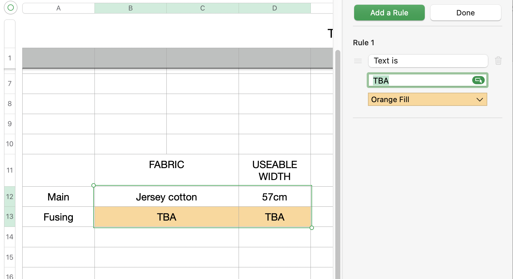
If you want "TBA" to always mean "additional information required from client', add this Conditional Highlighting rule to every cell that could contain TBA with this meaning:

Text is "TBA"

Orange Fill

This will give these cells an orange fill if the cell contains TBA, and Wayne's formula, revised to count only cells containing "TBA" will insert the 'orange print message if the count of 'TBA' cells is greater than zero.

Adding the revised formula, shown at the bottom of the screen shot below, to cell G10 shows the 'orange' message when there are cells in the selected area containing TBA.

And removes the message when there are no cells i the selected range containing TBA:

Text version of formula that can be copied, then pasted into the formula editor.

IF(COUNTIF(B12:D13,"TBA")>0,"ORANGE CELL = CLIENT TO PROVIDE MISSING INFORMATION", "")

Regards,

Barry

I cannot see you column headers and think that:

the 4 input cells are:

B12, D12

B13, D13

and the cell where the conditional message is to reside is G10

Select G10, then type, or copy and paste from here, then formula:

=IF(COUNTA(B12:D13)<4, "ORANGE CELL = CLIENT TO PROVIDE MISSING INFORMATION", "")

shorthand for this is:

G10=IF(COUNTA(B12:D13)<4, "ORANGE CELL = CLIENT TO PROVIDE MISSING INFORMATION", "")

remove the "=" sign from the beginning of the formula. if you select the cell and type what I pasted, then the formula will enter correctly. If you type the = to start dating a formula and then paste the formula I posted (including the =) you will get this result.

the operation is:

single click the cell

paste the formula

type return

A possible formula for your cell that says the customer needs to enter data:

=IF(COUNTA($A12:$A18)=COUNTIFS($A12:$A18,"<>",B12:B18,"<>",D12:D18,"<>"),"","Customer needs to enter data")

Reads: count the number of cells in column A that are filled in. Count the number of cells where columns A, B, and D are all filled in. If these two counts are equal than all data has been entered. If not then customer needs to enter data.

I suspect you are getting a 'self reference' error.

The range A2 to J18 includes the cell H10, which is the cell containing the formula.

The range should contain only the cells where TBA might be entered.

Regards,

Barry

Seeing Barry's post, the use of TBA makes it all a lot simpler than what I was doing. Better to go with that approach.