Apple Numbers Range of Data

H2 = ROW()

Fill down to complete the column

You can hide this column later.

G2 =IF(MAXIFS(H,A,"<="&E2,B,">="&E2,C,"<="&F2,D,">="&F2)>0,"In Stock", "Not In Stock")

You can fill down but if you only have one of each widget, you should only do one search at a time because if two searches require the same widget, only one is actually in stock.

You could do without column H if you replace the H in the formula with B or D. But if you keep column H, you can easily have the formula tell you which row the widget is in.

="ROW "&MAXIFS(H,A,"<="&E2,B,">="&E2,C,"<="&F2,D,">="&F2)

This will give you an answer like "Row 10" if in stock or "Row 0" if not. Conditional highlighting could be used to hide the "Row 0" or make it red text.

Oh, I get you now: for a dimension in Input Width and Input Height, you want to look up the whole table to see if at least one row would “fit” the input dimensions.

A solution would to split the existing table into two: one only containing the list, the other to do the search. Assume the 2nd table is named “Search Table”. Then in table “Data Table”, input this formula in E2 (The column E could be named “Fits”):

IF(AND(Search Table::A1>=A2, Search Table::A1<=B2, Search Table::B1>=C2, Search Table::B1<=D2), TRUE, FALSE)

A1 and B1 in “Search Table” would contain the “Input Width” and “Input Height”, respectively. Copy the formula in E2 to all the rows in column E. You could hide column E if you don’t want to display it.

Then, in table “Search Table”, in cell C1, use the formula:

IF(COUNTIF(Data Table:E, TRUE)>=1, “In Stock”, “Custom Build”)

Sorry, I didn't anticipate that you'd look for several items at the same time in the Search Table. The formula is valid for just one row in the Search Table. Copying it wouldn't work. I'm not sure how to get around this requirement.

One solution, if you limit the number of rows in Search Table, would be to add a new column in Data Table for each row you'd want. For instance, to implement a 2nd row in Search Table, the formulas would be:

In Data Table, column F:

IF(AND(Search Table::A2>=A2, Search Table::A2<=B2, Search Table::B2>=C2, Search Table::B2<=D2), TRUE, FALSE)

(see how the referenced cells are now Search Table::A2 and Search Table::B2, instead of Search Table::A1 and Search Table::A1 respectively.)

In Search Table, cell C2:

IF(COUNTIF(Data Table:F, TRUE)>=1, “In Stock”, “Custom Build”)

(see how the cell now references column F in Data Table, instead of column E.)

This solution could become burdensome if you intend to have a lot of rows in Search Table. If you decide to use it, I would suggest to limit the number of rows in Search Table by deleting the unneeded rows, so that another user would not be tempted to use more rows than intended, and thus get the wrong result.

I'll try to explain my pivot table. There are a couple of phases.

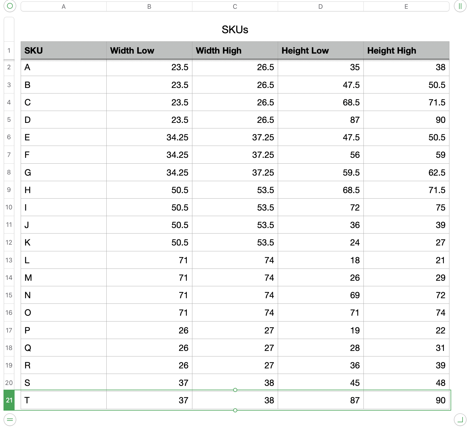
First off, I somewhat recreated your table of sizes, but added an additional 'SKU' column that identifies the specific standard model. This can really be anything, but is used as the key:

From here, I created a Pivot Table (Select the table, then Organize -> Create Pivot Table -> On New Sheet).

Because Numbers makes some assumptions on how you want to summarize the data, the initial table will be junk, but a simple cleanup will take care of that.

The important thing to remember is that pivot tables work by categorizing the rows and columns from the source table. You need to provide hints as to how you want them summarized.

This is done in the Organize sidebar when looking at the Pivot Table.

This is how I set mine up:

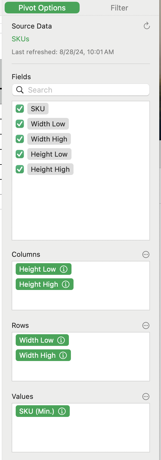
The main considerations are:

Fields: This is the list of fields from the source table that you want to summarize (the labels are taken from the header row of the table). I have all of them selected.

You then identify the row and column parameters. For this I've added the heights (low and high) in the Columns, and the widths (low and high) in the Rows section.

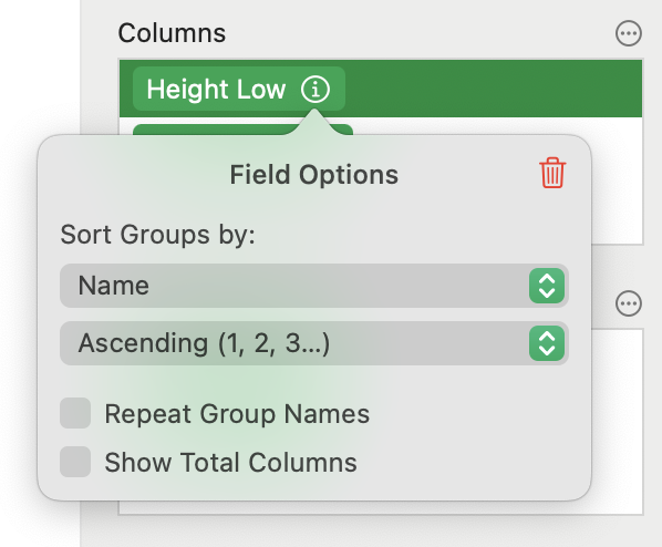
One additional change here is that we don't need to total the dimensions, so for each of the first entires in the Column and Row sections, Ctrl-click the entry and select Show Field Options, then turn off the 'Show Total Columns' option:

Finally, you tell it what data to summarize. For this, I set the SKU.

Now you should have a magic table that looks something like:

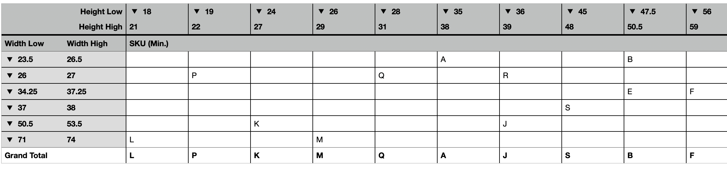
Here you can see the table has summarized the various width and height combinations, marking which SKU matches. Where there isn't a match, the cell is empty, but where there is a match it identifies the SKU for the corresponding widget.

Now it's just a matter of simple(-ish)lookups. Back to the main sheet.

I created an input table where you enter the desired width and height values:

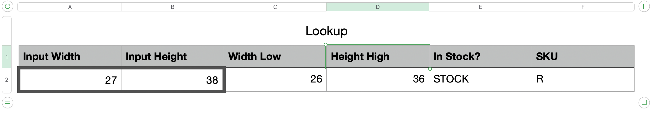
The idea here is that you enter the width and height.

For simplicity's sake I've broken it into a couple of steps to show the process, but it could be done in a single step by combining the formulas.

The important parts are:

Cell C2 = XLOOKUP($A2,SKUs::Width Low,SKUs::Width Low,"0",-1,1)

(should look like:

This performs a lookup in the SKU table using cell A2 (input width) to find the next smallest value.

A similar formula in cell D2 performs the lookup on the next smallest height value:

D2=XLOOKUP(B2,Height Low,Height Low,"0",-1,1)

This should dynamically locate the next-smallest value for each of the width and height values.

Now we can perform the lookup in the pivot table.

Cell F2= GETPIVOTDATA(SKU Pivot::$C$3,SKU Pivot::$C$3,SKU Pivot::$A$3,C2,SKU Pivot::$B$1,D2)

This takes the values in C2 and D2 and performs a lookup in the Pivot table. It will either return the SKU of the corresponding widget, or it will return 0 for no match.

Finally, I have cell E2:

E2=IF(ISTEXT(F2),"STOCK", "Custom Order")

Which checks if F2 (the PivotTable lookup) returns text or not, and sets to 'STOCK' or 'Custom Order' as appropriate. For grins, I also added conditional highlighting on this cell to show Custom Order as red text to highlight it.

Happy to send you my worksheet if recreating it from this diatribe is too much :)

I solved this a slightly different way - using a Pivot Table.

a Pivot Table essentially works out every possible combination. You can then use =GETPIVOTDATA to perform a lookup on that table given a width and height parameter. Any match will return the specific line item that matches, any non-match can return 0 (or not found).

It's hard to describe how to setup a pivot table here, though, but it's worth checking into.

You can also use MINIFS. If there is more than one match, MAXIFS will give you the last match in the table (the one with the highest row number), MINIFS will give you the first (lowest row number) match in the table.

You could use the AND() function. For instance:

IF(AND(E2>=A2, E2<=B2, F2>=C2, F2<=D2), “In Stock”, “Custom Build”)