Apple launches Apple Store app in India

The Apple Store app provides customers with the most personalized way to shop for Apple’s innovative lineup of products and services. Learn more >

You can make a difference in the Apple Support Community!

When you sign up with your Apple Account, you can provide valuable feedback to other community members by upvoting helpful replies and User Tips.

Looks like no one’s replied in a while. To start the conversation again, simply ask a new question.

Highlight a cell based on condition of another

Example:

I want B4 to Highlight if B4 is ticked. That's it and I can't seem to do it, conditional highlighting does not seem to do it and I have nor do formula from what any solution seems complicated for a simple requirement. Can you help?

iMac 24″, macOS 13.5

Posted on Sep 10, 2023 10:05 AM

Reply
Question marked as Top-ranking reply

Posted on Sep 10, 2023 2:47 PM

There is no direct way to do it but it can be done with an additional column. There are a couple of ways to do it. I took your question one step further in the example below to do two colors. The method shown lets you conditional highlight the entire row if you want to.
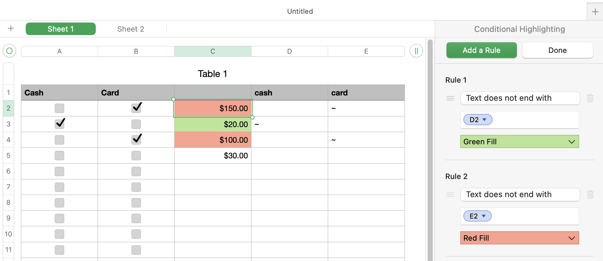


If you don't want to do two colors, you can follow the steps below except don't put a formula in column D, don't make the rule that refers to column D, and, when it is all set up, delete column D.


D2 =IF(A2,"~","")

E2 =IF(B2,"~","")

fill down to complete the columns


Creating the highlighting rules for the cells in column C

  1. Select column C (select all cells that will get the rules, not headers and not usually footers).
  2. Start to create a conditional highlighting rule of "text does not end with"
  3. In the box where you would type in that text is a green oval. Click it.
  4. Click on cell D2
  5. Click the green checkmark to accept your selection
  6. Choose the color/style you want for the rule
  7. Add another rule
  8. Do same as above except this time click on E2


Cell C2 will get rules using D2 and E2. C3 will get rules using D3 and E3, etc.


If you want to highlight the entire row (including the checkboxes), not just column C, you would do this instead:

  1. Select columns A-C (all the cells that will get the rules)
  2. Do same as in the steps above except after selecting cell D2, edit it so it is $D2.
  3. Same for E2, make it $E2


Hide the extra columns when it is all set up and working.


I usually use CHAR(10000) instead of "~" for this but "~" is simpler (as suggested by SGIII). The important thing is the character cannot be something that any of your "text" might actually end with.


3 replies
Question marked as Top-ranking reply

Sep 10, 2023 2:47 PM in response to JCB@89050

There is no direct way to do it but it can be done with an additional column. There are a couple of ways to do it. I took your question one step further in the example below to do two colors. The method shown lets you conditional highlight the entire row if you want to.


If you don't want to do two colors, you can follow the steps below except don't put a formula in column D, don't make the rule that refers to column D, and, when it is all set up, delete column D.


D2 =IF(A2,"~","")

E2 =IF(B2,"~","")

fill down to complete the columns


Creating the highlighting rules for the cells in column C

  1. Select column C (select all cells that will get the rules, not headers and not usually footers).
  2. Start to create a conditional highlighting rule of "text does not end with"
  3. In the box where you would type in that text is a green oval. Click it.
  4. Click on cell D2
  5. Click the green checkmark to accept your selection
  6. Choose the color/style you want for the rule
  7. Add another rule
  8. Do same as above except this time click on E2


Cell C2 will get rules using D2 and E2. C3 will get rules using D3 and E3, etc.


If you want to highlight the entire row (including the checkboxes), not just column C, you would do this instead:

  1. Select columns A-C (all the cells that will get the rules)
  2. Do same as in the steps above except after selecting cell D2, edit it so it is $D2.
  3. Same for E2, make it $E2


Hide the extra columns when it is all set up and working.


I usually use CHAR(10000) instead of "~" for this but "~" is simpler (as suggested by SGIII). The important thing is the character cannot be something that any of your "text" might actually end with.


Highlight a cell based on condition of another

Welcome to Apple Support Community
A forum where Apple customers help each other with their products. Get started with your Apple Account.